Jacobian of the LTC transformation

My recent paper builds on this Linearly Transformed Cosines paper by Eric Heitz. Infact, this was a collaboration with Eric himself! Linearly Tranformed Cosines or LTCs are a transformation of the rendering integral under specific assumptions, which lead to analytic solutions of it. One of the outcomes of my new work was the relaxation of the isotropic assumption of LTCs, allowing the use of anisotropic BRDFs.

Although I have read the original paper countless times and worked on an extension of it, I still was puzzled by the LTC jacobian derivation given in the appendix of the original paper:

The derivation must be pretty obvious to a lot of people but to me it wasn’t so. This post is an attempt to give a detailed and intuitive derivation of this expression (Eq. 18 above). Why is this important? Well, in my view small details like these expand your horizon, and you can only hope to get new ideas if you throughly understand what’s already out there. Also, its always fun to understand things from a mathematical perspective, even if you are a intuitive-first person like I am.

I would like to note that figures in this post have been directly taken from the original paper.

Definitions

Its best if you have read and are confortable with Eric’s original paper. However, I am still defining things here to ensure consistency.

Direction vectors on the unit sphere are given by $\omega =(x,y,z)$. $D_o({\omega }_o)$ is the source (clamped cosine) distribution. $D(\omega )$ is the target (~ GGX BRDF) distribution. Given an LTC matrix $M$, the direction vectors $\omega$ of $D$ are obtained by from the direction vectors ${\omega }_o$ of $D_o$ by:

$$\omega =\frac{M{\omega }_o}{||M{\omega }_o||}.$$

The magnitude at the transformed direction is given by:

$$\boxed{{\displaystyle D(\omega )=D_o({\omega }_o)\frac{\partial {\omega }_o}{\partial \omega }.}}$$

Here, $\frac{\partial {\omega }_o}{\partial \omega }$ is the determinant of jacobian of the transformation (which is frequently referred to as just the jacobian). This is what we will derive in this post.

Another thing we will find useful is the solid angle subtended by a small facet having area $A$, which is given by:

$$\partial \omega =\frac{A(\hat{r}\cdot \hat{n})}{r^2},$$

where $\partial \omega$ is a small solid angle, $\hat{r}$ is the normalized position vector of the facet, $\hat{n}$ is the surface normal of the facet and $r^2$ is the distance to the facet.

Finally, we will find use of the cross product under linear transforms property:

$$M{\omega }_1\times M{\omega }_2=|M|M^{-T}({\omega }_1\times {\omega }_2)=|M|M^{-T}{\omega }_o$$

Derivation

First things first. Note that $D$ and $D_o$ are distributions in 2D, although they appear to be distributions in 3D. To see why, note that these are distributions on the unit sphere. Hence, we can write $\omega =(\sin \theta \cos \varphi ,\sin \theta \sin \varphi ,\cos \theta )$, in turn making $D$ and $D_o$ dependent on only $\theta ,\varphi$ (thus two dimensional).

From the definition of jacobian determinants, $\frac{\partial {\omega }_o}{\partial \omega }$ measures how a differential area around ${\omega }_o$ changes. Since this differential area in on the unit sphere, it is basically the solid angle. The LTC jacobian thus measures change in solid angle under the LTC transform.

Our problem now boils down to determining how a differential solid angle changes under $M$.

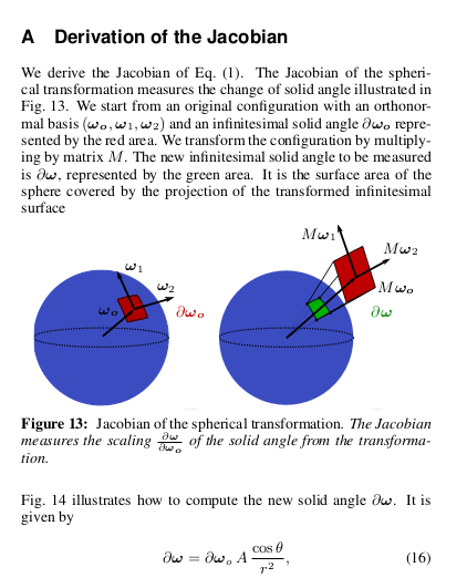
Let’s take the differential solid angle $\partial {\omega }_o$ in $D_o$. Since this is small enough, it can also be considered as a planar facet. Now, define two vectors ${\omega }_1,{\omega }_2$, which together with ${\omega }_o$ form an orthonormal basis. (Figure 2, left)

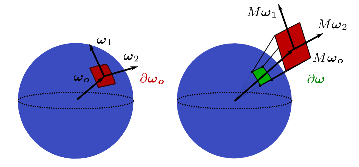
Transforming these vectors by LTC $M$ results in a new set of vectors (Figure 2, right). The area of the facet $\partial {\omega }_o$ is now changed to $\partial {\omega }_o\cdot A$, where $A$ is the area of parallelogram defined by vectors $M{\omega }_1$ and $M{\omega }_2$.

A subtelty you may want to note, is that in Figure 2 left, the area of the parallelogram given by ${\omega }_1$ and ${\omega }_2$ is $1$, thus the differential area is only $\partial {\omega }_o$. This changes in Figure 2 right, since the area of the parallelogram is not $1$ anymore, and thus the differential area is $\partial {\omega }_o\cdot A$.

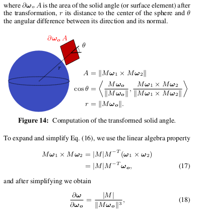
Alright! Now how about the differential solid angle $\partial \omega$ after the LTC transform? Its essentialy the solid angle subtended by a small facet! We know this directly (see definitions section):

$$\partial \omega =\frac{\partial {\omega }_{o}A(\hat{r}\cdot \hat{n})}{r^2}.$$

The terms $\hat{r},\hat{n}$ and $A$ are simple to define in this case.

The area is $A=\Vert M{\omega }_1\times M{\omega }_2\Vert$, which is a standard formula.

The unit position vector is $\hat{r}=\frac{M{\omega }_o}{\Vert M{\omega }_o\Vert }$ (the division just normalizes since $\hat{r}$ is a unit vector).

And finally, the normal vector is $\hat{n}=\frac{M{\omega }_1\times M{\omega }_2}{\Vert M{\omega }_1\times M{\omega }_2\Vert }$ (again, division for normalization).

Lets first simplify the dot product $\hat{r}\cdot \hat{n}$ by plugging in the above definitions:

$$\hat{r}\cdot \hat{n}={\left(\frac{M{\omega }_o}{\Vert M{\omega }_o\Vert }\right)}^T\frac{M{\omega }_1\times M{\omega }_2}{\Vert M{\omega }_1\times M{\omega }_2\Vert }$$

Using coss product under linear transforms property:

$$\hat{r}\cdot \hat{n}=\frac{(M{\omega }_o{)}^T}{\Vert M{\omega }_o\Vert }\frac{|M|M^{-T}{\omega }_o}{\Vert M{\omega }_1\times M{\omega }_2\Vert }$$ $$=\frac{|M|(M{\omega }_o{)}^T{M}^{-T}{\omega }_o}{\Vert M{\omega }_o\Vert \Vert M{\omega }_1\times M{\omega }_2\Vert }$$

Using the fact that $(M{\omega }_o{)}^T={\omega }_o^T{M}^T$:

$$=\frac{|M|{\omega }_o^T{M}^T{M}^{-T}{\omega }_o}{\Vert M{\omega }_o\Vert \Vert M{\omega }_1\times M{\omega }_2\Vert }$$ $$=\frac{|M|{\omega }_o^T{\omega }_o}{\Vert M{\omega }_o\Vert \Vert M{\omega }_1\times M{\omega }_2\Vert }$$

${\omega }_o^T{\omega }_o$ is equal to $1$, since ${\omega }_o$ is a unit vector.

$$⟹\hat{r}\cdot \hat{n}=\frac{|M|}{\Vert M{\omega }_o\Vert \Vert M{\omega }_1\times M{\omega }_2\Vert }$$

Finally, substitue into and simplify the expression for $\partial \omega$:

$$\partial \omega =\frac{\partial {\omega }_{o}A(\hat{r}\cdot \hat{n})}{r^2}$$ $$\frac{\partial \omega }{\partial {\omega }_o}=\frac{A(\hat{r}\cdot \hat{n})}{r^2}$$ $$⟹\frac{\partial \omega }{\partial {\omega }_o}=\frac{\Vert M{\omega }_1\times M{\omega }_2\Vert }{\Vert M{\omega }_o{\Vert }^2}\frac{|M|}{\Vert M{\omega }_o\Vert \Vert M{\omega }_1\times M{\omega }_2\Vert }$$ $$\boxed{{\displaystyle ⟹\frac{\partial \omega }{\partial {\omega }_o}=\frac{|M|}{\Vert M{\omega }_o{\Vert }^3}.}}$$

This is what we are looking for!

Conclusion

This is a pretty intuitive proof, given that you think and go about it the right way. Hope this post helps some of you in your own research journey!